Background
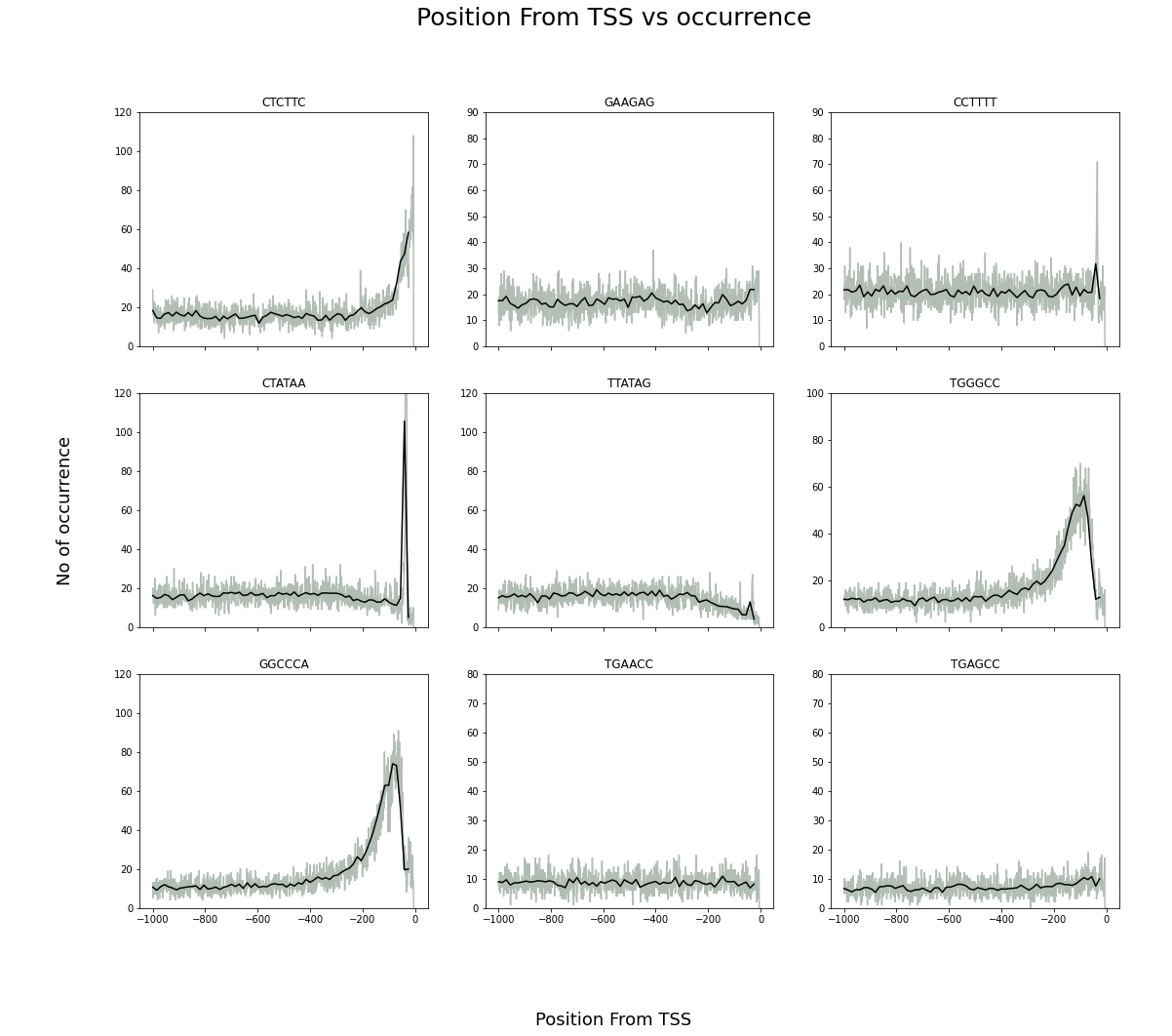
In my first month at cBLAST, I was given a task to reproduce figure 1 and figure 2 of “Identification of plant promoter constituents by analysis of local distribution of short sequences” to enhance my skill. From the work of Yamamoto, Y.Y. et al., LDSS (Local Distribution of Short Sequences) have been identified within promoters of Arabidopsis thaliana and Oryza Sativa.1. I tried to reproduce their findings using python code. Here goes my produced figures and code.
Patterns of distribution of peaks
First I used a dictionary of dictionaries where the key of the first dictionary is all possible hexamers. The value against a kmer (hexamer) is another dictionary whose key is distance from TSS (Transcription Start Site) and value is the number of occurrences of that kmer in Oryza Sativa genome. I also created a similar dictionary of dictionaries for average/windowed values of 15 base pairs. Finally, plotted location vs occurrences plot in matplotlib.subplots.

Code:
First let’s import the libraries
import matplotlib.pyplot as plt
from Bio import SeqIO
import numpy as np

#global variables
ShortSeqLen = 6
One utility function I use to find all possible kmers. Let me know if you find any usefull one. Let’s also initialize the dictionary.
def AllPossibleKmers(k):
    '''Provides a list of all possible kmers'''
    lst = ['A', 'G','T','C']
    for j in range(k-1):
        lst = lst* 4
        for i in range(0,int(len(lst)/4)):
            lst[i]+='A'
        for i in range(int(len(lst)/4),int(len(lst)/2)):
            lst[i]+='G'
        for i in range(int(len(lst)/2),int(3*len(lst)/4)):
            lst[i]+='T'
        for i in range(int(3*len(lst)/4),int(len(lst))):
            lst[i]+='C'
    return lst

localdistributions = dict()
for kmer in AllPossibleKmers(ShortSeqLen):
    localdistributions[kmer] = dict()
    for i in range(-1000,0,1):
        localdistributions[kmer][i] = 0
Updating the dictionary from the genome of Oryza sativa.
fasta_sequences = SeqIO.parse(open('IRGSP-1.0_1kb-upstream_2021-11-11.fasta'),'fasta')
for fasta in fasta_sequences:
    name, promoter = fasta.id, str(fasta.seq)
    # got each promoter
    for i in range (-1000,0-ShortSeqLen+1,1):
        ShortSeq = promoter[1000+i: 1000+i+ShortSeqLen]
        ShortSeq = ShortSeq.upper()
        #print(i,ShortSeq,end='\n ')
        if ShortSeq in localdistributions:
            localdistributions[ShortSeq][i] += 1
        #else:
            #print('ShortSeq is not found in Local Distribution Dictionary')

localdistributions_windowed = dict()
for kmer in AllPossibleKmers(ShortSeqLen):
    localdistributions_windowed[kmer] = dict()
    for i in range(-1000+7,0,15):
        sum = 0
        for j in range(i-7,i+8,1):
            if j == -5:
                break
            sum+= localdistributions[kmer][j]
        localdistributions_windowed[kmer][i] = sum/15
Ploting the resut
fig, ax = plt.subplots(3,3,sharex=True,figsize=(18, 15))
fig.suptitle("Fig 1. Position From TSS vs occurrence",fontsize=25)
fig.supxlabel('Position From TSS',fontsize=18)
fig.supylabel('No of occurrence',fontsize=18)

ax[0][0].plot(localdistributions['CTCTTC'].keys(),localdistributions['CTCTTC'].values(),color='#B2BEB5')
ax[0][0].plot(localdistributions_windowed['CTCTTC'].keys(),localdistributions_windowed['CTCTTC'].values(),color='#000')
ax[0][0].set_title('CTCTTC')
ax[0][0].set_ylim([0,120])
Peak Analysis and Finding Peak positive Hexamers
For peak analysis the following parameters were used:
Relative Peak Area (RPA) = Peak Area/total area;
Relative Peak Height (RPH) = peak height/Base Line;
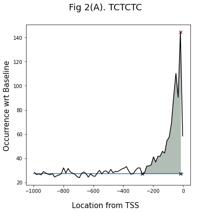
Peak Area/basal fluctuation = Peak Area/∆area per peak width, ∆area represents the grey area.
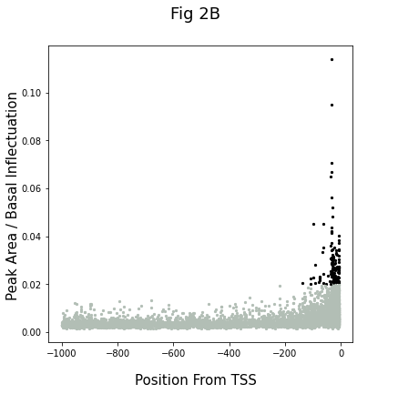
The graph (2B) shows the results. Each dot shows the data of an individual hexamer. The kmers having Peak Area/basal fluctuation > 0.2 were identified as LDSS positive. They can be further classified into three groups, pyrimidine patch (Y Patch), TATA box, and REG (Regulatory Element Group) 1


code for peak analysis:
def PABFandPeakPosition_exact(ShortSeq):
    #finding base
    base = 0
    for i in range(-993,-499,15):       # upto -498
        base += localdistributions_windowed[ShortSeq][i]
    base/=33
    #exact calculation
    exact_peak_height = 0
    exact_peak_position = ''

    for i in range(-1000,0-ShortSeqLen,1):
        if localdistributions[ShortSeq][i] > exact_peak_height:
            exact_peak_height = localdistributions[ShortSeq][i]
            exact_peak_position = i

    #print('Peak height: ',peak_height,'Peak Position: ',peak_position)

    peak_r = exact_peak_position
    while localdistributions[ShortSeq][peak_r] > base and peak_r + 1 < 0-ShortSeqLen:
        peak_r += 1

    peak_l = exact_peak_position
    while localdistributions[ShortSeq][peak_l] > base and peak_l-1 > -1000:
        peak_l -= 1


    exact_peak_width = abs(peak_r - peak_l)

    #approximate calculation
    peak_height = 0
    peak_position = ''

    for i in range(-993,0-ShortSeqLen,15):
        if localdistributions_windowed[ShortSeq][i] > peak_height:
            peak_height = localdistributions_windowed[ShortSeq][i]
            peak_position = i

    #print('Peak height: ',peak_height,'Peak Position: ',peak_position)

    peak_r = peak_position
    while localdistributions_windowed[ShortSeq][peak_r] > base and peak_r + 15 < 0-ShortSeqLen:
        peak_r += 15

    peak_l = peak_position
    if peak_l < -1000:
        peak_l += 15
    while localdistributions_windowed[ShortSeq][peak_l] > base and peak_l-15 > -1000:
        peak_l -= 15


    peak_width = abs(peak_r - peak_l)
    #print('Peak_l',peak_l,'peak_r',peak_r, 'Peak Width', peak_width)

    peak_elements_x = list()
    for i in range(peak_l, peak_r+1, 15):
        peak_elements_x.append(i)

    peak_elements_y = list()
    for i in peak_elements_x:
        peak_elements_y.append(localdistributions_windowed[ShortSeq][i])

    #print('Relative Peak Hight =',peak_height/base)
    peak_std = np.std(peak_elements_y)


    total_area = 0
    for i in range(-993,0-ShortSeqLen,15):
        total_area += (abs(localdistributions_windowed[ShortSeq][i]-base)+abs(localdistributions_windowed[ShortSeq][i+15]-base))*0.5
    total_area*=15

    grey_area = 0
    for i in range(-993,-500,15):
        grey_area += (abs(localdistributions_windowed[ShortSeq][i]-base)+abs(localdistributions_windowed[ShortSeq][i+15]-base))*0.5
    grey_area*=15

    peak_area =0
    for i in range(peak_l,peak_r-15+1,15):
        peak_area += (abs(localdistributions_windowed[ShortSeq][i]-base)+abs(localdistributions_windowed[ShortSeq][i+15]-base))*0.5
    peak_area*=15

    #print('total area =',total_area, '\nPeak area =',peak_area, '\ngrey area =',grey_area)
    #print('Relative Peak Area =',peak_area / total_area)
    #print('Peak Area / Basal Flactuation =', peak_area/(grey_area*peak_width))
    return peak_area/(grey_area*peak_width), exact_peak_position
ploting result:
fig, ax = plt.subplots(figsize=(6, 6))
fig.suptitle("Fig 2B",fontsize=18)
fig.supxlabel('Position From TSS',fontsize=15)
fig.supylabel('Peak Area / Basal Inflectuation',fontsize=15)
for ShortSeq in AllPossibleKmers(ShortSeqLen):
    PAbyBF,PeakPosition = PABFandPeakPosition_exact(ShortSeq)
    if PAbyBF >= 0.02:
        ax.scatter(PeakPosition,PAbyBF,color='#000',s=5)
    else:
        ax.scatter(PeakPosition,PAbyBF,color='#B2BEB5',s=5)
My remarks
Writing the code was the easiest part, but reading the paper again and again to find out what they did and how they did cost most of the time. This project might not be that difficult or technically important but I still wanted to write it as a blog post, since it was my first task at cBLAST. I am looking forward to working on more projects or tasks that involve the promoter region.
References
-
Yamamoto, Y.Y., Ichida, H., Matsui, M. et al. Identification of plant promoter constituents by analysis of local distribution of short sequences. BMC Genomics 8, 67 (2007). https://doi.org/10.1186/1471-2164-8-67 ↩ ↩2